Lecture 1 — Introduction & Tools

Data & Code Management: From Collection to Application

Samuel Orso

2025-09-25

Welcome!

Course: Data & Code Management: From Collection to Application
Time & place: Thursdays 9:00–12:00
Communication: Slack (class workspace)
Materials: GitHub repo & website
Grading: participation (bonus), homeworks (3 indivuals) and final project (group)
Always refer to the course website dcm.samorso.ch for the latest info!

“Reproducibility is job #1 for modern data science.”
— everyone who has ever lost a script 😉

Note

Today’s goals
1. Understand course scope & expectations
2. See why reproducibility matters
3. Meet the core toolchain (R, Python, SQL, GitHub, Markdown/Jupyter/Quarto)
4. Try small, focused exercises

Agenda

Course overview & evaluation
Reproducibility in analytics
Core tools & workflows
Quarto refresher
GitHub refresher
Mini‑exercises

Tip: Slides include short activities you can try during/after class.

Course Overview

Orientation: hands‑on data & code practices for analytics
You will:
- write clean R/Python code
- query data via SQL
- document with Markdown/Jupyter/Quarto
- use Git/GitHub (branches, PRs, issues)
- deliver a reproducible project (group)
We value: clarity, collaboration, curiosity

Tip

Success checklist
- Commit early, commit often
- Make small, reversible changes
- Automate what repeats
- Document decisions, not only code
- Prefer scripts & notebooks over manual clicks

Expectations & Evaluation

Participation: engaged presence (practicals), Slack questions/answers
Homeworks: short, targeted (programming, SQL, tooling)
Project: real‑world style, reproducible deliverable
Academic integrity: cite sources, no copy‑paste answers

Tools allowed: R, Python, SQL, Quarto, GitHub, AI copilots (with provenance & verification).

What are LLMs?

Definition: Large Language Models (LLMs) are AI models trained on vast amounts of text data to understand and generate human language.
Examples:
- GPT-4, GPT-5 (OpenAI)
- Gemini (Google)
- LLaMA (Meta)
- Claude (Anthropic)
Capabilities:
- Natural language understanding and generation
- Text completion, summarization, translation
- Assistance in various domains, including programming.

Why are they important for programming?

LLMs can understand code as a special type of language.
They offer assistance in code generation, debugging, and improving programming productivity.

LLM for Programming - Key Features

Code Suggestions:
- Automates repetitive coding tasks.
- Helps in writing boilerplate code.
- See for instance GitHub’s copilot.
Error Debugging:
- Identifies and resolves bugs in code snippets.
- Suggests alternative solutions or optimizations.
Code Explanation:
- Breaks down complex code into simple explanations.
- Helps in learning new programming concepts.

Benefits of Using LLMs like ChatGPT in Programming

1. Increased Productivity

Automates repetitive and boilerplate tasks.
Helps explore new coding approaches faster.

2. Learning and Discovery

Explains code, libraries, and new languages in an intuitive manner.
Great for beginners and advanced users alike.

Challenges and Considerations

1. Not Always Correct

LLMs can suggest incorrect code, it can hallucinate, requiring human oversight.

2. Context Limitations

LLMs lack the full project context, so they might not understand the specific requirements.

3. Ethical Concerns

Intellectual property, security, and data privacy must be considered when using AI for programming.

Important

AI policy (short)
Use AI to brainstorm, outline, or lint code. Own the result: verify outputs, write your tests, and document AI assistance (what, why, where).

Minimal Project Structure

project/
├─ data/           # raw/ and processed/ (never overwrite raw)
├─ R/ or src/      # functions, modules
├─ notebooks/      # exploratory analysis
├─ reports/        # Quarto/Markdown outputs
├─ tests/          # unit tests
├─ renv/ or .venv/ # R or Python environment
├─ .gitignore
└─ README.md

Tooling Map

R (tidyverse, data.table) & Python (pandas, polars)
SQL for data retrieval/joins/aggregations (week 5)
Git + GitHub for versioning & collaboration
Markdown/Jupyter/Quarto for literate workflows
Optional helpers: make, pre-commit, linters

R snippet

# Vectorized transform
library(dplyr)
set.seed(42)
df <- tibble(x = rnorm(5), y = rnorm(5))
df |>
  mutate(z = x + y, grp = if_else(z > 0, "pos", "neg"))

Python snippet

import pandas as pd
import numpy as np
rng = np.random.default_rng(42)
df = pd.DataFrame({"x": rng.normal(size=5), "y": rng.normal(size=5)})
df.assign(z=lambda d: d.x + d.y,
          grp=lambda d: np.where(d.z > 0, "pos", "neg"))

Caution

Are these codes reproducible? Why/why not?

Literate Programming with Quarto

Write text + code together
Render to HTML/PDF/slides/reports
Parametrized reports & caching
Works with R and Python

plot(mtcars$wt, mtcars$mpg)

Render:

quarto render report.qmd

Important

House rule: every analysis step appears in a script/notebook—no manual spreadsheet edits.

What is Quarto?

Quarto: successor of RMarkdown
markdown contrasts markup languages (e.g. HTML) which require heavy syntax
Quarto provides a literate programming framework for data science.
Literate programming: narrative + code in the same document.
Reproducible research: analyses can be reproduced the same way by someone else.

What is Quarto?

In a nutshell, Quarto builds on Pandoc and execution engines (Knitr for R, Jupyter for Python/Julia/Observable). It allows embedding code into Markdown documents, which can be rendered into multiple formats (HTML, PDF, Word, …).

Create a Quarto document

In RStudio or VSCode, click File → New File → Quarto Document. Or simply create a .qmd file.

Important features of `markdown`

Three aspects:
- YAML metadata
- Text
- Code cells/chunks

YAML (YAML Ain’t Markup Language)

Header where options are defined.
Surrounded by ---
Options include: author, date, output format, table of contents, themes, code folding, …

Example:

---
title: "My Report"
author: "Jane Doe"
format: html
toc: true
---

Text in Markdown

Core body, essential for explaining your analysis.
Markdown syntax:
- *italics*, **bold**, code style
- headers (#, ##, ###)
- lists (*, -, +, 1.)
- links: [Quarto](https://quarto.org)
- blockquotes (> …)
- images: ![](path/to/img.png)
- tables (basic Markdown or functions like knitr::kable())

Extended text features

Math: in $\LaTeX$ via $...$ inline or $$...$$ display.
Cross-references: @fig-label or @sec-label.
Citations with .bib files ([@doe2023]).
You can always use HTML when needed.

Code cells in Quarto

Quarto supports R, Python, Julia, and ObservableJS.

Code cell delimiters:

```r
# R code here
```

```python
# Python code here
```

In Jupyter notebooks, the same concepts apply — each code cell is language-specific.

Chunk / cell options

Quarto syntax uses YAML-like #| comments:

```r
#| echo: false
#| eval: true
#| warning: false
#| cache: false
1 + 1
```

Options you’ll use most often:

eval: run code?
echo: show code?
warning: show warnings?
cache: reuse computations?

Figures in code cells

Options for plots:

```r
#| fig-width: 6
#| fig-height: 4
#| fig-align: center
#| fig-cap: "A scatterplot"
plot(iris$Sepal.Length, iris$Sepal.Width)
```

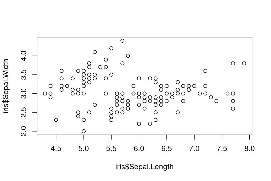
A scatterplot

Printing tables with `knitr::kable()`

```r
#| echo: true
#| fig-height: 5
data("iris")
knitr::kable(iris[1:5,])
```

Sepal.Length	Sepal.Width	Petal.Length	Petal.Width	Species
5.1	3.5	1.4	0.2	setosa
4.9	3.0	1.4	0.2	setosa
4.7	3.2	1.3	0.2	setosa
4.6	3.1	1.5	0.2	setosa
5.0	3.6	1.4	0.2	setosa

For enhanced tables: kableExtra.

Extended tables with `kableExtra`

library(kableExtra)
mtcars[1:3, 1:8] %>%
  kbl() %>%
  kable_paper(full_width = T)

	mpg	cyl	disp	hp	drat	wt	qsec	vs
Mazda RX4	21.0	6	160	110	3.90	2.620	16.46	0
Mazda RX4 Wag	21.0	6	160	110	3.90	2.875	17.02	0
Datsun 710	22.8	4	108	93	3.85	2.320	18.61	1

Mathpix for equations

Mathpix Snip digitizes handwritten/printed math and pastes directly into Markdown/LaTeX/Word.

Live preview

RStudio: quarto preview
VSCode: Quarto extension
Jupyter: live interactive editing

Instant feedback without full rebuilds.

Version Control with GitHub

Why GitHub?

Work with others on the same project without endless email exchanges
Avoid “file_v1”, “file_v2”, “final_version_really.R” chaos
Track who changed what and when
Discuss, review, and plan changes in one place

Tip

💡 Think of GitHub as both a time machine and a teamwork hub.

Why GitHub for this course?

We will use GitHub to:
- Work in groups on projects
- Submit homeworks
- Develop programs

What is Git?

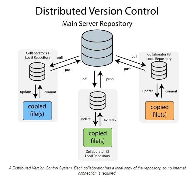
Git is a distributed version control system:

Distributed: every copy of a project has the full history
Version control: keeps track of all changes to your project

Important

Instead of dozens of “final” files, Git records every change in one clean history.

Types of Version Control Systems

Local – on your own computer
Centralized – one main server (risk of failure!)
Distributed – full history on every machine (Git)

Why Version Control?

Collaborate safely with others
Roll back mistakes
Explore new ideas with branches
Reduce risks of file loss or corruption

Git ≠ GitHub

Git = software for version control
GitHub = website/platform that hosts Git repositories
Alternatives: GitLab, BitBucket, SourceForge

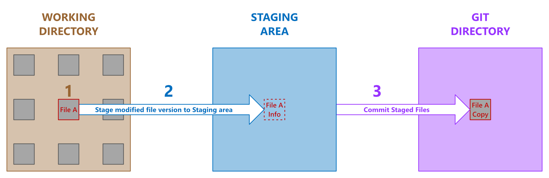
File States in Git

A file can be:
- Untracked – new, not in Git yet
- Modified – changed, not saved in history
- Staged – marked for next snapshot
- Committed – safely stored in the repository

Ignoring Files

Use a .gitignore file to tell Git which files to skip:
- Temporary files (.Rhistory, .DS_Store)
- Large data files
- Secrets or keys

GitHub: Basic Workflow

Open your RStudio project (linked to GitHub)
Work locally as usual
Save often
Commit snapshots of your changes
Push commits to GitHub
On another computer (or from a teammate) → Pull updates

Tip

Always pull before you push to avoid conflicts!

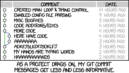
Commits

Commit = snapshot of your work
Good commit messages explain why you changed something, not just what

Common Issues & Fixes

Wrong repo → Double-check you’re in the right project
Large files (>100MB) → use another service (Dropbox, Zenodo, etc.)
Conflicts → someone else changed the same file → git pull --rebase
Merge conflicts → same lines changed → talk to your teammate + edit manually

New Habits with GitHub

Commit often
Push regularly
Pull before you start working
Communicate with teammates

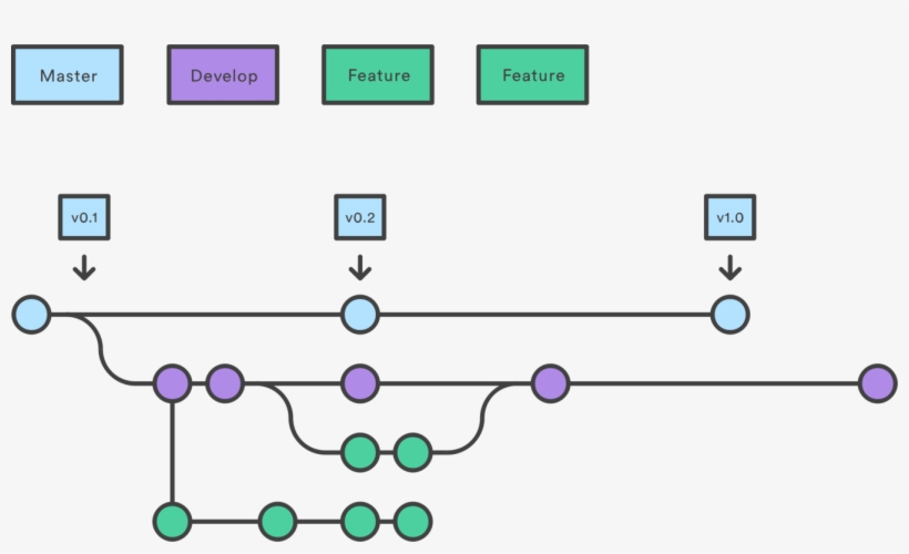
Collaboration Rituals

Branch → small PR → peer review → merge
Use Issues with labels (“bug”, “enhancement”, “question”)
Templates: PULL_REQUEST_TEMPLATE.md, ISSUE_TEMPLATE.md
Document decisions in CHANGELOG.md

Note

Activity (2’): In pairs, outline a PR description for adding a new utils/plot.R with one function and one test.

Example PR Description

PR Title
Add utils/plot.R with basic plotting function and test

Summary
- Add plot_scatter() in utils/plot.R
- Add test in tests/testthat/test-plot.R

Details
- Input validation (numeric vectors of equal length)
- Uses ggplot2
- Tests:
- Error if unequal lengths
- Output is "ggplot"

Example PR Description (cont.)

Checklist
- [x] Function implemented
- [x] Tests added
- [x] Documentation with roxygen2
- [ ] CI checks pass

Related Issues
Closes #12 (feature request: plotting utilities)

GitHub in a Nutshell

Git gets easier once you get the basic idea that branches are homeomorphic endofunctors mapping submanifolds of a Hilbert space.
—Isaac Wolkerstorfer (joking)

Git in 6 commands

git status
git add -A
git commit -m "Explain what/why, not how"
git pull --rebase
git push
git switch -c feature/your-topic   # create a feature branch

Note

Activity (think‑pair‑share):
What makes a good commit message? Write one for “fixed weird bug in script” that would help your future self.

Reproducibility in Practice

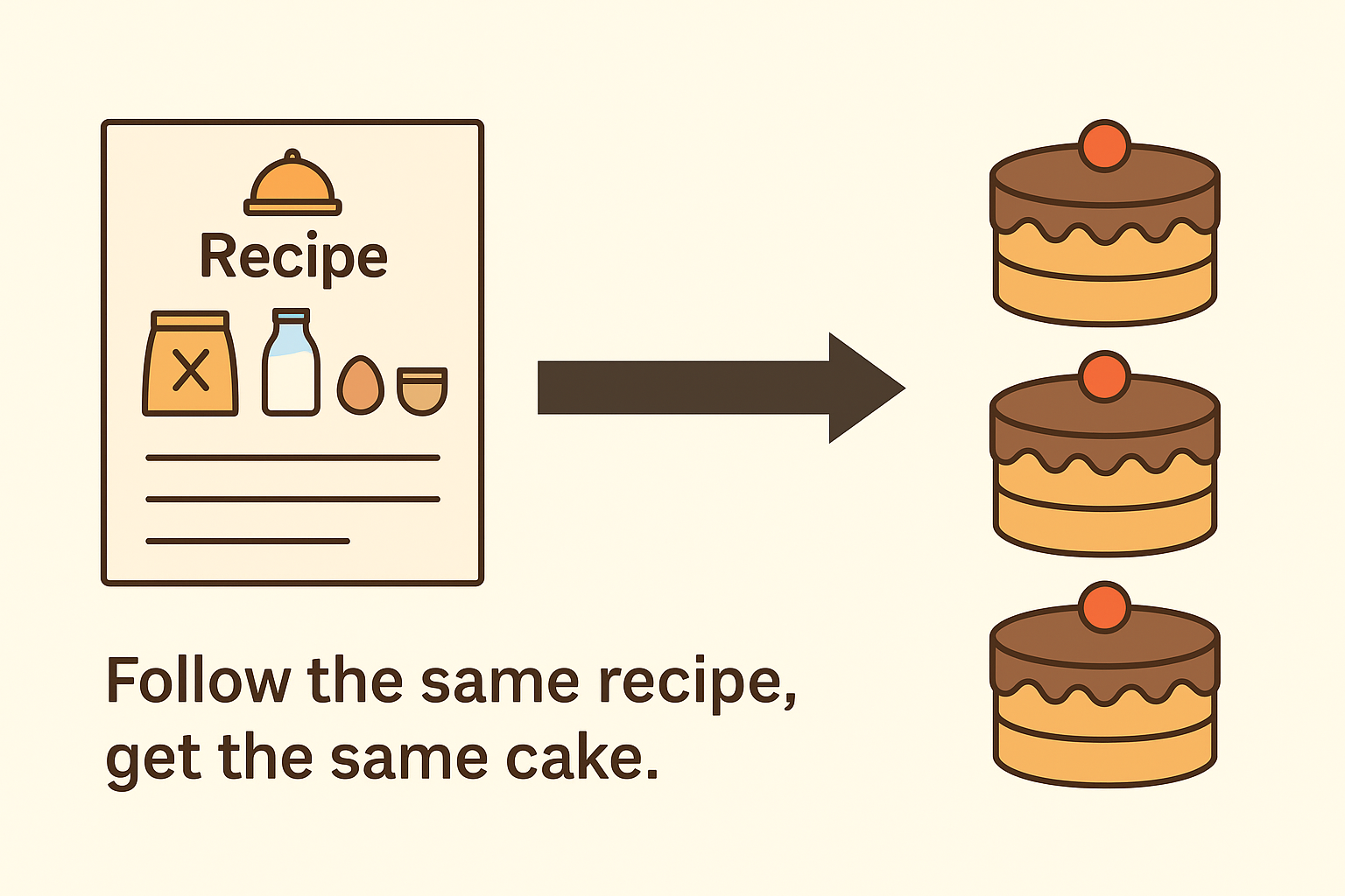
Reproducibility: Why it matters

Symptoms of non‑reproducible work (raise your hand if you’ve seen these):
- “It works on my machine.”
- “I changed nothing and it broke.”
- “Which file is the final_final_v3.R?”

Principles
- Deterministic environments
- Versioned code and data contracts
- Scripts, not clicks
- Single‑source of truth (parameters, config)
- Literate programming (Markdown/Quarto)
- Automated checks (CI later in course)

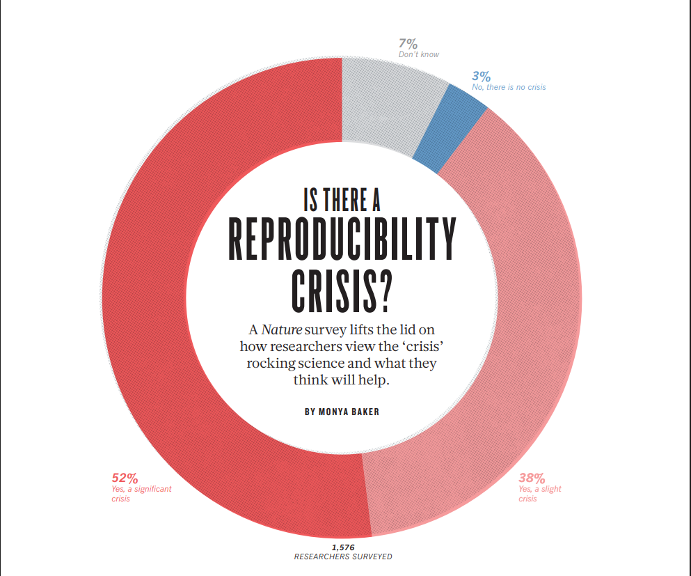
Is there a reproducibility crisis?

Environments (determinism)

R — renv

install.packages("renv")
renv::init()
renv::snapshot()   # lock versions
renv::restore()    # reproduce elsewhere

Python — Conda (recommended)

# create & activate
conda create -n bia python=3.11 pandas scikit-learn jupyterlab -c conda-forge
conda activate bia

# share exact env
conda env export --from-history > environment.yml
# reproduce elsewhere
conda env create -f environment.yml

Python — Poetry (alternative)

# once
poetry config virtualenvs.in-project true
# in project
poetry init
poetry add pandas scikit-learn jupyter
poetry install           # recreate from poetry.lock

Note

Exercise (1′): List one package you rely on in R and in Python. Why lock its version?

Nondeterminism in LLM

Reproducibility is a bedrock of scientific progress. However, it’s remarkably difficult to get reproducible results out of large language models.
Horace He in collaboration with others at Thinking Machines

Note

Read the full article here

Data Contracts & File Hygiene

Never overwrite raw/ data
Validate schemas (columns, types, keys)
Record data provenance (source, timestamp)
Use .gitignore to avoid committing large/secret files

# data & local env
data/raw/*
!.gitkeep
.venv/
renv/library/
*.sqlite
*.parquet

Common Pitfalls & How to Avoid Them

Undocumented notebooks → add titles, goals, outputs
Hidden state (globals) → pass parameters explicitly (next lecture)
One giant script → split into modules
No seeds → set seeds where randomness matters
Unpinned packages → lock versions

Quick Wins You Can Adopt Today

Create a project with folders from the template earlier
Initialize Git and push to GitHub
Set up renv or .venv or equivalent
Convert one analysis to Quarto

What’s Next

Next lecture: Programming foundations (R & Python)
Before next time: ensure you can
1. clone a GitHub repo,
2. create a branch & commit,
3. render a Quarto .qmd to HTML,
4. set up renv or .venv.

Tip

If stuck: ask on Slack—show error, steps tried, and minimal example.

Mini-exercise (1): R

Open RStudio (or your preferred IDE).
Create a new R script named exercise1.R.
Write R code that:
1. Creates a numeric vector of length 5.
2. Computes its mean.
3. Prints the result with a short message.

Note

💡 Tip: Use c() for vectors, mean() for averages, and paste() for printing messages.

Mini-exercise (2): Python

Create a new Python file named exercise2.py.
Write a script that:
1. Creates a list of 5 numbers.
2. Computes their average.
3. Prints the result.

Note

💡 Tip: Use sum() and len() to calculate an average.

Mini-exercise (3): Quarto

Create a new Quarto document named exercise3.qmd.
Add:
- A title and author.
- One R code chunk that prints "Hello R!".
- One Python code chunk that prints "Hello Python!".
Render the document to HTML.

Note

💡 Tip: Use ```{r} and ```{python} for chunks.

Mini-exercise (4): GitHub

Create a new GitHub repository called first-exercises.
Add the three files you created (exercise1.R, exercise2.py, exercise3.qmd).
Write a short README.md describing what each file does.
Commit and push your changes.

Note

💡 Tip: Use GitHub Desktop, git on the command line, or RStudio’s Git interface.

Mini-exercise (5): R + Data

In R, load the built-in dataset mtcars.
Compute the average miles per gallon (mpg) by the number of cylinders (cyl).
Make a simple scatterplot of mpg vs hp (horsepower).
Save the script as exercise5.R.

Note

💡 Tip: Look at aggregate() or dplyr::group_by() + summarise(). Use plot() for a quick scatterplot.

Mini-exercise (6): Python + Visualization

In Python, use the pandas and matplotlib libraries.
Load the dataset iris (you can import it from sklearn.datasets).
Compute the average petal length per species.
Make a histogram of sepal lengths.
Save the script as exercise6.py.

Note

💡 Tip: pandas.DataFrame.groupby() is useful for summaries.

Mini-exercise (7): Quarto + Reproducibility

Create a Quarto document called exercise7.qmd.
Include:
- A title, author, and date.
- A short text section explaining what the document does.
- One R chunk producing a table of summary statistics (e.g., summary(mtcars)).
- One Python chunk producing a plot of the iris dataset.
Render both HTML and PDF versions.

Note

💡 Tip: To render PDF, you may need LaTeX installed. Use quarto render exercise7.qmd --to pdf.

Mini-exercise (8): All Together 🎯

Create a new Quarto document named exercise8.qmd.
Inside it:
- Add a short introduction paragraph.
- An R chunk that computes and prints the mean of mtcars$mpg.
- A Python chunk that loads iris and plots sepal length vs sepal width.
Render the document to HTML.
Push the .qmd, the HTML output, and any supporting files to your GitHub repo first-exercises.
Update your README.md to include a short description of this integrated exercise.

Note

💡 Goal: Practice combining R + Python code in Quarto, and making results reproducible via GitHub.

💡 Bonus Opportunity

If you prepare a solution to one of the mini-exercises
and present it briefly during the next practical session
👉 You may receive a bonus point (participation credit).

Note

🌟 Tip: The focus is on sharing your approach, not on having a perfect solution.

Q&A

Thanks!
Optional: After class, try converting one old analysis to Quarto and push it to GitHub with a short README.

Solution (1): R

# exercise1.R
x <- c(3, 7, 9, 2, 5)
m <- mean(x)
message(paste("The mean is", m))

Solution (2): Python

# exercise2.py
nums = [3, 7, 9, 2, 5]
avg = sum(nums) / len(nums)
print(f"The average is {avg}")

Solution (3): Quarto

---
title: "Exercise 3"
author: "Your Name"
format: html
---

```r
"Hello R!"
```

```python
print("Hello Python!")
```

Solution (4): GitHub

# In a fresh folder:
git init
git branch -M main
git remote add origin https://github.com/<user>/first-exercises.git

# Add files
git add exercise1.R exercise2.py exercise3.qmd README.md
git commit -m "Add first three exercises"
git push -u origin main

Example README.md:

# first-exercises
- `exercise1.R`: vector + mean (R)
- `exercise2.py`: list + average (Python)
- `exercise3.qmd`: R & Python chunks (Quarto)

Solution (5): R + Data

# exercise5.R
# A. summary by cylinders
aggregate(mpg ~ cyl, data = mtcars, FUN = mean)

# Using dplyr (optional)
# library(dplyr)
# mtcars |>
#   group_by(cyl) |>
#   summarise(mean_mpg = mean(mpg))

# B. scatterplot mpg vs hp
plot(mtcars$hp, mtcars$mpg,
     xlab = "Horsepower (hp)", ylab = "Miles per gallon (mpg)",
     main = "mtcars: mpg vs hp")

Solution (6): Python + Visualization

# exercise6.py
import pandas as pd
import matplotlib.pyplot as plt
from sklearn.datasets import load_iris

# Load iris
iris_bunch = load_iris(as_frame=True)
df = iris_bunch.frame  # columns: sepal length (cm), sepal width (cm), ...
df["species"] = df["target"].map(dict(enumerate(iris_bunch.target_names)))

# Average petal length per species
avg_petal = df.groupby("species")["petal length (cm)"].mean()
print(avg_petal)

# Histogram of sepal lengths
plt.figure()
df["sepal length (cm)"].hist()
plt.title("Histogram: Sepal Length")
plt.xlabel("Sepal length (cm)")
plt.ylabel("Count")
plt.tight_layout()
plt.show()

Solution (7): Quarto + Reproducibility

---
title: "Exercise 7"
author: "Your Name"
format:
  html: default
  pdf: default
---

This document shows basic R summaries and a Python plot.

```r
summary(mtcars)
```

```python
import matplotlib.pyplot as plt
from sklearn.datasets import load_iris
iris = load_iris(as_frame=True).frame
plt.figure()
plt.scatter(iris["sepal length (cm)"], iris["sepal width (cm)"])
plt.title("Iris: Sepal length vs width")
plt.xlabel("Sepal length (cm)")
plt.ylabel("Sepal width (cm)")
plt.tight_layout()
plt.show()
```

Render:

quarto render exercise7.qmd --to html
quarto render exercise7.qmd --to pdf   # requires LaTeX

Solution (8): All Together 🎯

---
title: "Exercise 8 (Capstone)"
author: "Your Name"
format: html
---

This Quarto file combines R + Python and is tracked on GitHub.

```r
mean(mtcars$mpg)
```

```python
from sklearn.datasets import load_iris
import matplotlib.pyplot as plt
iris = load_iris(as_frame=True).frame
plt.figure()
plt.scatter(iris["sepal length (cm)"], iris["sepal width (cm)"])
plt.title("Iris: Sepal length vs width")
plt.xlabel("Sepal length (cm)")
plt.ylabel("Sepal width (cm)")
plt.tight_layout()
plt.show()
```

Push results:

quarto render exercise8.qmd
git add exercise8.qmd exercise8.html
git commit -m "Add capstone exercise with R+Python"
git push

Lecture 1 — Introduction & Tools

Welcome!

Agenda

Course Overview

Expectations & Evaluation

What are LLMs?

Why are they important for programming?

LLM for Programming - Key Features

Benefits of Using LLMs like ChatGPT in Programming

1. Increased Productivity

2. Learning and Discovery

Challenges and Considerations

1. Not Always Correct

2. Context Limitations

3. Ethical Concerns

Minimal Project Structure

Tooling Map

Literate Programming with Quarto

What is Quarto?

What is Quarto?

Create a Quarto document

Important features of markdown

YAML (YAML Ain’t Markup Language)

Text in Markdown

Extended text features

Code cells in Quarto

Chunk / cell options

Figures in code cells

Printing tables with knitr::kable()

Extended tables with kableExtra

Mathpix for equations

Live preview

Version Control with GitHub

Why GitHub?

Why GitHub for this course?

What is Git?

Types of Version Control Systems

Why Version Control?

Git ≠ GitHub

File States in Git

Ignoring Files

GitHub: Basic Workflow

Commits

Common Issues & Fixes

New Habits with GitHub

Collaboration Rituals

Example PR Description

Example PR Description (cont.)

GitHub in a Nutshell

Git in 6 commands

Reproducibility in Practice

Reproducibility: Why it matters

Is there a reproducibility crisis?

Environments (determinism)

Nondeterminism in LLM

Data Contracts & File Hygiene

Common Pitfalls & How to Avoid Them

Quick Wins You Can Adopt Today

What’s Next

Mini-exercise (1): R

Mini-exercise (2): Python

Mini-exercise (3): Quarto

Mini-exercise (4): GitHub

Mini-exercise (5): R + Data

Mini-exercise (6): Python + Visualization

Mini-exercise (7): Quarto + Reproducibility

Mini-exercise (8): All Together 🎯

💡 Bonus Opportunity

Q&A

Solution (1): R

Solution (2): Python

Solution (3): Quarto

Solution (4): GitHub

Solution (5): R + Data

Solution (6): Python + Visualization

Solution (7): Quarto + Reproducibility

Solution (8): All Together 🎯

Important features of `markdown`

Printing tables with `knitr::kable()`

Extended tables with `kableExtra`